
Databases using SQL
Setup
- Install Firefox
- Install the SQLite Manager add on Tools -> Add-ons -> Search -> SQLite Manager -> Install -> Restart
- Download the Portal Database
- Open SQLite Manage Firefox Button -> Web Developer -> SQLite Manager
Relational databases
- Relational databases store data in tables with fields (columns) and records (rows)
- Data in tables has types, just like in Python, and all values in a field have the same type (list of data types)
- Queries let us look up data or make calculations based on columns
- The queries are distinct from the data, so if we change the data we can just rerun the query
Database Management Systems
There are a number of different database management systems for working with relational data. We're going to use SQLite today, but basically everything we teach you will apply to the other database systems as well (e.g., MySQL, PostgreSQL, MS Access, Filemaker Pro). The only things that will differ are the details of exactly how to import and export data and the details of data types.
The data
This is data on a small mammal community in southern Arizona over the last 35 years. This is part of a larger project studying the effects of rodents and ants on the plant community. The rodents are sampled on a series of 24 plots, with different experimental manipulations of which rodents are allowed to access the plots.
This is a real dataset that has been used in over 100 publications. I've simplified it just a little bit for the workshop, but you can download the full dataset and work with it using exactly the same tools we'll learn about today.
Database Design
- Order doesn't matter
- Every row-column combination contains a single atomic value, i.e., not containing parts we might want to work with separately.
- One field per type of information
- No redundant information
- Split into separate tables with one table per class of information
- Needs an identifier in common between tables – shared column - to reconnect (foreign key).
Import
- Start a New Database Database -> New Database
- Start the import Database -> Import
- Select the file to import
- Give the table a name (or use the default)
- If the first row has column headings, check the appropriate box
- Make sure the delimiter and quotation options are correct
- Press OK
- When asked if you want to modify the table, click OK
- Set the data types for each field
EXERCISE: Import the plots and species tables
You can also use this same approach to append new data to an existing table.
Basic queries
Let's start by using the surveys table. Here we have data on every individual that was captured at the site, including when they were captured, what plot they were captured on, their species ID, sex and weight in grams.
Let’s write an SQL query that selects only the year column from the surveys table.
SELECT year FROM surveys;
We have capitalized the words SELECT and FROM because they are SQL keywords. SQL is case insensitive, but it helps for readability – good style.
If we want more information, we can just add a new column to the list of fields, right after SELECT:
SELECT year, month, day FROM surveys;
Or we can select all of the columns in a table using the wildcard *
SELECT * FROM surveys;
Unique values
If we want only the unique values so that we can quickly see what species have
been sampled we use DISTINCT
SELECT DISTINCT species FROM surveys;
If we select more than one column, then the distinct pairs of values are returned
SELECT DISTINCT year, species FROM surveys;
Calculated values
We can also do calculations with the values in a query. For example, if we wanted to look at the mass of each individual on different dates, but we needed it in kg instead of g we would use
SELECT year, month, day, wgt/1000.0 from surveys
When we run the query, the expression wgt / 1000.0 is evaluated for each row
and appended to that row, in a new column. Expressions can use any fields, any
arithmetic operators (+ - * /) and a variety of built-in functions (). For
example, we could round the values to make them easier to read.
SELECT plot, species, sex, wgt, ROUND(wgt / 1000.0, 2) FROM surveys;
EXERCISE: Write a query that returns The year, month, day, speciesID and weight in mg
Filtering
Databases can also filter data – selecting only the data meeting certain criteria. For example, let’s say we only want data for the species Dipodomys merriami, which has a species code of DM. We need to add a WHERE clause to our query:
SELECT * FROM surveys WHERE species="DM";
We can do the same thing with numbers. Here, we only want the data since 2000:
SELECT * FROM surveys WHERE year >= 2000;
We can use more sophisticated conditions by combining tests with AND and OR. For example, suppose we want the data on Dipodomys merriami starting in the year 2000:
SELECT * FROM surveys WHERE (year >= 2000) AND (species = "DM");
Note that the parentheses aren’t needed, but again, they help with readability. They also ensure that the computer combines AND and OR in the way that we intend.
If we wanted to get data for any of the Dipodomys species, which have species codes DM, DO, and DS we could combine the tests using OR:
SELECT * FROM surveys WHERE (species = "DM") OR (species = "DO") OR (species = "DS");
EXERCISE: Write a query that returns The day, month, year, species ID, and weight (in kg) for individuals caught on Plot 1 that weigh more than 75 g
Saving & Exporting results
- Exporting: Actions button and choosing Save Result to File.
- Save: View drop down and Create View
Saving queries
To enable saving queries from the main menu select Tools -> Use Table for Extension Data:
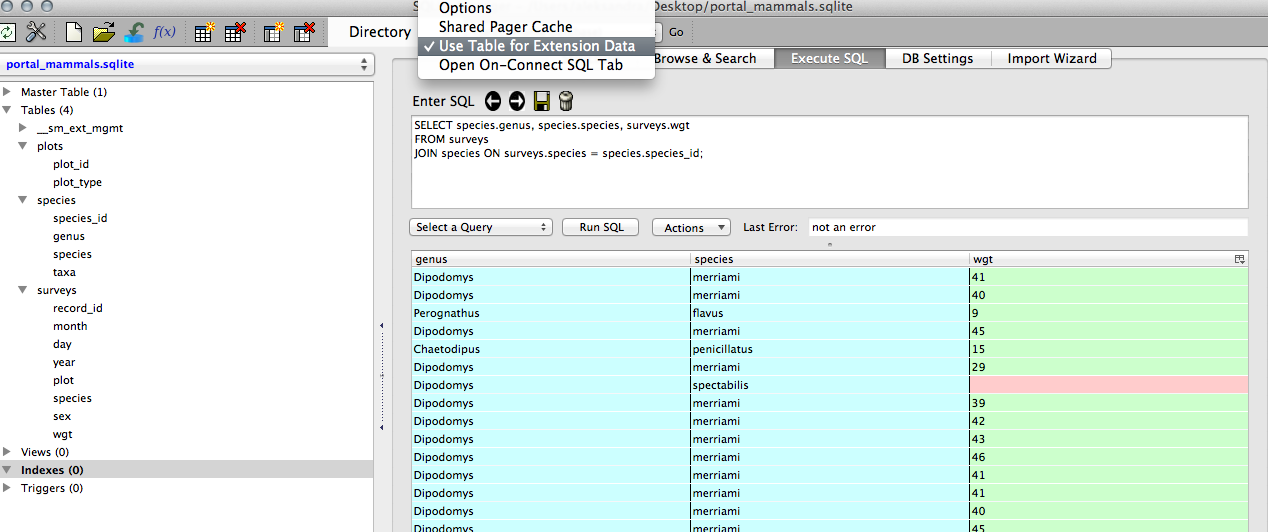
You will see additional 4 icons - "Previous query from the history", "Next query from the history", "Save query by name" and "Clear query history". When you click the query, it will then be available under the list of queries ("Select a Query").
Building more complex queries
Now, lets combine the above queries to get data for the 3 Dipodomys species from
the year 2000 on. This time, let’s use IN as one way to make the query easier
to understand. It is equivalent to saying WHERE (species = "DM") OR (species
= "DO") OR (species = "DS"), but reads more neatly:
SELECT * FROM surveys WHERE (year >= 2000) AND (species IN ("DM", "DO", "DS"));

SELECT *
FROM surveys
WHERE (year >= 2000) AND (species IN ("DM", "DO", "DS"));
We started with something simple, then added more clauses one by one, testing their effects as we went along. For complex queries, this is a good strategy, to make sure you are getting what you want. Sometimes it might help to take a subset of the data that you can easily see in a temporary database to practice your queries on before working on a larger or more complicated database.
Sorting
We can also sort the results of our queries by using ORDER BY. For simplicity, let’s go back to the species table and alphabetize it by taxa.
SELECT * FROM species ORDER BY taxa ASC;
The keyword ASC tells us to order it in Ascending order. We could alternately use DESC to get descending order.
SELECT * FROM species ORDER BY taxa DESC;
ASC is the default.
We can also sort on several fields at once. To truly be alphabetical, we might want to order by genus then species.
SELECT * FROM species ORDER BY genus ASC, species ASC;
Exercise: Write a query that returns year, species, and weight in kg from the surveys table, sorted with the largest weights at the top
Order of execution
Another note for ordering. We don’t actually have to display a column to sort by it. For example, let’s say we want to order by the species ID, but we only want to see genus and species.
SELECT genus, species FROM species ORDER BY taxon ASC;
We can do this because sorting occurs earlier in the computational pipeline than field selection.
The computer is basically doing this:
- Filtering rows according to WHERE
- Sorting results according to ORDER BY
- Displaying requested columns or expressions.
Order of clauses
The order of the clauses when we write a query is dictated by SQL: SELECT, FROM, WHERE, ORDER BY and we often write each of them on their own line for readability.
Exercise: Let's try to combine what we've learned so far in a single query. Using the surveys table write a query to display the three date fields, species ID, and weight in kilograms (rounded to two decimal places), for rodents captured in 1999, ordered alphabetically by the species ID.
Aggregation
Aggregation allows us to combine results by grouping records based on value and calculating combined values in groups.
Let’s go to the surveys table and find out how many individuals there are. Using the wildcard simply counts the number of records (rows)
SELECT COUNT(*) FROM surveys
We can also find out how much all of those individuals weigh.
SELECT COUNT(*), SUM(wgt) FROM surveys
Do you think you could output this value in kilograms, rounded to 3 decimal places?
SELECT ROUND(SUM(wgt)/1000.0, 3) FROM surveys
There are many other aggregate functions included in SQL including MAX, MIN, and AVG.
From the surveys table, can we use one query to output the total weight, average weight, and the min and max weights? How about the range of weight?
Now, let's see how many individuals were counted in each species. We do this using a GROUP BY clause
SELECT species, COUNT(*)
FROM surveys
GROUP BY species
GROUP BY tells SQL what field or fields we want to use to aggregate the data. If we want to group by multiple fields, we give GROUP BY a comma separated list.
EXERCISE: Write queries that return: 1. How many individuals were counted in each year *2. Average weight of each species in each year
We can order the results of our aggregation by a specific column, including the aggregated column. Let’s count the number of individuals of each species captured, ordered by the count
SELECT species, COUNT(*)
FROM surveys
GROUP BY species
ORDER BY COUNT(species)
Joins
To combine data from two tables we use the SQL JOIN command, which comes after the FROM command.
We also need to tell the computer which columns provide the link between the two tables using the word ON. What we want is to join the data with the same species codes.
SELECT *
FROM surveys
JOIN species ON surveys.species = species.species_id
ON is like WHERE, it filters things out according to a test condition. We use the table.colname format to tell the manager what column in which table we are referring to.
We often won't want all of the fields from both tables, so anywhere we would have used a field name in a non-join query, we can use table.colname
For example, what if we wanted information on when individuals of each species were captured, but instead of their species ID we wanted their actual species names.
SELECT surveys.year, surveys.month, surveys.day, species.genus, species.species
FROM surveys
JOIN species ON surveys.species = species.species_id
Exercise: Write a query that returns the genus, the species, and the weight of every individual captured at the site
Joins can be combined with sorting, filtering, and aggregation. So, if we wanted average mass of the individuals on each different type of treatment, we could do something like
SELECT plots.plot_type, AVG(surveys.wgt)
FROM surveys
JOIN plots
ON surveys.plot = plots.plot_id
GROUP BY plots.plot_type
Adding data to existing tables
- Browse & Search -> Add
- Enter data into a csv file and append
Other database management systems
- Access or Filemaker Pro
- GUI
- Forms w/QAQC
- But not cross-platform
- MySQL/PostgreSQL
- Multiple simultaneous users
- More difficult to setup and maintain
Q & A on Database Design (review if time)
- Order doesn't matter
- Every row-column combination contains a single atomic value, i.e., not containing parts we might want to work with separately.
- One field per type of information
- No redundant information
- Split into separate tables with one table per class of information
- Needs an identifier in common between tables – shared column - to reconnect (foreign key).
Data types
| Data type | Description |
|---|---|
| CHARACTER(n) | Character string. Fixed-length n |
| VARCHAR(n) or CHARACTER VARYING(n) | Character string. Variable length. Maximum length n |
| BINARY(n) | Binary string. Fixed-length n |
| BOOLEAN | Stores TRUE or FALSE values |
| VARBINARY(n) or BINARY VARYING(n) | Binary string. Variable length. Maximum length n |
| INTEGER(p) | Integer numerical (no decimal). |
| SMALLINT | Integer numerical (no decimal). |
| INTEGER | Integer numerical (no decimal). |
| BIGINT | Integer numerical (no decimal). |
| DECIMAL(p,s) | Exact numerical, precision p, scale s. |
| NUMERIC(p,s) | Exact numerical, precision p, scale s. (Same as DECIMAL) |
| FLOAT(p) | Approximate numerical, mantissa precision p. A floating number in base 10 exponential notation. |
| REAL | Approximate numerical |
| FLOAT | Approximate numerical |
| DOUBLE PRECISION | Approximate numerical |
| DATE | Stores year, month, and day values |
| TIME | Stores hour, minute, and second values |
| TIMESTAMP | Stores year, month, day, hour, minute, and second values |
| INTERVAL | Composed of a number of integer fields, representing a period of time, depending on the type of interval |
| ARRAY | A set-length and ordered collection of elements |
| MULTISET | A variable-length and unordered collection of elements |
| XML | Stores XML data |
SQL Data Type Quick Reference
Different databases offer different choices for the data type definition.
The following table shows some of the common names of data types between the various database platforms:
| Data type | Access | SQLServer | Oracle | MySQL | PostgreSQL |
|---|---|---|---|---|---|
| boolean | Yes/No | Bit | Byte | N/A | Boolean |
| integer | Number (integer) | Int | Number | Int / Integer | Int / Integer |
| float | Number (single) | Float / Real | Number | Float | Numeric |
| currency | Currency | Money | N/A | N/A | Money |
| string (fixed) | N/A | Char | Char | Char | Char |
| string (variable) | Text (<256) / Memo (65k+) | Varchar | Varchar / Varchar2 | Varchar | Varchar |
| binary object OLE Object Memo Binary (fixed up to 8K) | Varbinary (<8K) | Image (<2GB) Long | Raw Blob | Text Binary | Varbinary |