Analyzing Patient Data

We are studying inflammation in patients who have been given a new treatment for arthritis, and need to analyze the first dozen data sets. The data sets are stored in comma-separated values (CSV) format: each row holds information for a single patient, and the columns represent successive days. The first few rows of our first file look like this:

0,0,1,3,1,2,4,7,8,3,3,3,10,5,7,4,7,7,12,18,6,13,11,11,7,7,4,6,8,8,4,4,5,7,3,4,2,3,0,0
0,1,2,1,2,1,3,2,2,6,10,11,5,9,4,4,7,16,8,6,18,4,12,5,12,7,11,5,11,3,3,5,4,4,5,5,1,1,0,1
0,1,1,3,3,2,6,2,5,9,5,7,4,5,4,15,5,11,9,10,19,14,12,17,7,12,11,7,4,2,10,5,4,2,2,3,2,2,1,1
0,0,2,0,4,2,2,1,6,7,10,7,9,13,8,8,15,10,10,7,17,4,4,7,6,15,6,4,9,11,3,5,6,3,3,4,2,3,2,1
0,1,1,3,3,1,3,5,2,4,4,7,6,5,3,10,8,10,6,17,9,14,9,7,13,9,12,6,7,7,9,6,3,2,2,4,2,0,1,1

We want to:

• load that data into memory,
• calculate the average inflammation per day across all patients, and
• plot the result.

To do all that, we'll have to learn a little bit about programming.

Loading Data

Words are useful, but what's more useful are the sentences and stories we build with them. Similarly, while a lot of powerful tools are built into languages like Python, even more live in the libraries they are used to build.

In order to load our inflammation data, we need to import a library called NumPy. In general you should use this library if you want to do fancy things with numbers, especially if you have matrices. We can load NumPy using:

import numpy

Importing a library is like getting a piece of lab equipment out of a storage locker and setting it up on the bench. Once it's done, we can ask the library to read our data file for us:

numpy.loadtxt(fname='inflammation-01.csv', delimiter=',')

array([[ 0.,  0.,  1., ...,  3.,  0.,  0.],
       [ 0.,  1.,  2., ...,  1.,  0.,  1.],
       [ 0.,  1.,  1., ...,  2.,  1.,  1.],
       ..., 
       [ 0.,  1.,  1., ...,  1.,  1.,  1.],
       [ 0.,  0.,  0., ...,  0.,  2.,  0.],
       [ 0.,  0.,  1., ...,  1.,  1.,  0.]])

The expression numpy.loadtxt(...) is a function call that asks Python to run the function loadtxt that belongs to the numpy library. This dotted notation is used everywhere in Python to refer to the parts of things as thing.component.

numpy.loadtxt has two parameters: the name of the file we want to read, and the delimiter that separates values on a line. These both need to be character strings (or strings for short), so we put them in quotes.

When we are finished typing and press Shift+Enter, the notebook runs our command. Since we haven't told it to do anything else with the function's output, the notebook displays it. In this case, that output is the data we just loaded. By default, only a few rows and columns are shown (with ... to omit elements when displaying big arrays). To save space, Python displays numbers as 1. instead of 1.0 when there's nothing interesting after the decimal point.

Our call to numpy.loadtxt read our file, but didn't save the data in memory. To do that, we need to assign the array to a variable. A variable is just a name for a value, such as x, current_temperature, or subject_id. Python's variables must begin with a letter. We can create a new variable simply by assigning a value to it using =. As an illustration, let's step back and instead of considering a table of data, consider the simplest "collection" of data, a single value. The line below assigns a value to a variable:

weight_kg = 55

Once a variable has a value, we can print it:

print weight_kg

55

and do arithmetic with it:

print 'weight in pounds:', 2.2 * weight_kg

weight in pounds: 121.0

We can also change a variable's value by assigning it a new one:

weight_kg = 57.5
print 'weight in kilograms is now:', weight_kg

weight in kilograms is now: 57.5

As the example above shows, we can print several things at once by separating them with commas.

If we imagine the variable as a sticky note with a name written on it, assignment is like putting the sticky note on a particular value:

This means that assigning a value to one variable does not change the values of other variables. For example, let's store the subject's weight in pounds in a variable:

weight_lb = 2.2 * weight_kg
print 'weight in kilograms:', weight_kg, 'and in pounds:', weight_lb

weight in kilograms: 57.5 and in pounds: 126.5

and then change weight_kg:

weight_kg = 100.0
print 'weight in kilograms is now:', weight_kg, 'and weight in pounds is still:', weight_lb

weight in kilograms is now: 100.0 and weight in pounds is still: 126.5

Since weight_lb doesn't "remember" where its value came from, it isn't automatically updated when weight_kg changes. This is different from the way spreadsheets work.

Just as we can assign a single value to a variable, we can also assign an array of values to a variable using the same syntax. Let's re-run numpy.loadtxt and save its result:

data = numpy.loadtxt(fname='inflammation-01.csv', delimiter=',')

This statement doesn't produce any output because assignment doesn't display anything. If we want to check that our data has been loaded, we can print the variable's value:

print data

[[ 0.  0.  1. ...,  3.  0.  0.]
 [ 0.  1.  2. ...,  1.  0.  1.]
 [ 0.  1.  1. ...,  2.  1.  1.]
 ..., 
 [ 0.  1.  1. ...,  1.  1.  1.]
 [ 0.  0.  0. ...,  0.  2.  0.]
 [ 0.  0.  1. ...,  1.  1.  0.]]

Manipulating Data

Now that our data is in memory, we can start doing things with it. First, let's ask what type of thing data refers to:

print type(data)

<type 'numpy.ndarray'>

The output tells us that data currently refers to an N-dimensional array created by the NumPy library. We can see what its shape is like this:

print data.shape

(60, 40)

This tells us that data has 60 rows and 40 columns. data.shape is a member of data, i.e., a value that is stored as part of a larger value. We use the same dotted notation for the members of values that we use for the functions in libraries because they have the same part-and-whole relationship.

If we want to get a single value from the matrix, we must provide an index in square brackets, just as we do in math:

print 'first value in data:', data[0, 0]

first value in data: 0.0

print 'middle value in data:', data[30, 20]

middle value in data: 13.0

The expression data[30, 20] may not surprise you, but data[0, 0] might. Programming languages like Fortran and MATLAB start counting at 1, because that's what human beings have done for thousands of years. Languages in the C family (including C++, Java, Perl, and Python) count from 0 because that's simpler for computers to do. As a result, if we have an M×N array in Python, its indices go from 0 to M-1 on the first axis and 0 to N-1 on the second. It takes a bit of getting used to, but one way to remember the rule is that the index is how many steps we have to take from the start to get the item we want.

In the Corner

What may also surprise you is that when Python displays an array, it shows the element with index [0, 0] in the upper left corner rather than the lower left. This is consistent with the way mathematicians draw matrices, but different from the Cartesian coordinates. The indices are (row, column) instead of (column, row) for the same reason, which can be confusing when plotting data.

An index like [30, 20] selects a single element of an array, but we can select whole sections as well. For example, we can select the first ten days (columns) of values for the first four (rows) patients like this:

print data[0:4, 0:10]

[[ 0.  0.  1.  3.  1.  2.  4.  7.  8.  3.]
 [ 0.  1.  2.  1.  2.  1.  3.  2.  2.  6.]
 [ 0.  1.  1.  3.  3.  2.  6.  2.  5.  9.]
 [ 0.  0.  2.  0.  4.  2.  2.  1.  6.  7.]]

The slice 0:4 means, "Start at index 0 and go up to, but not including, index 4." Again, the up-to-but-not-including takes a bit of getting used to, but the rule is that the difference between the upper and lower bounds is the number of values in the slice.

We don't have to start slices at 0:

print data[5:10, 0:10]

[[ 0.  0.  1.  2.  2.  4.  2.  1.  6.  4.]
 [ 0.  0.  2.  2.  4.  2.  2.  5.  5.  8.]
 [ 0.  0.  1.  2.  3.  1.  2.  3.  5.  3.]
 [ 0.  0.  0.  3.  1.  5.  6.  5.  5.  8.]
 [ 0.  1.  1.  2.  1.  3.  5.  3.  5.  8.]]

We also don't have to include the upper and lower bound on the slice. If we don't include the lower bound, Python uses 0 by default; if we don't include the upper, the slice runs to the end of the axis, and if we don't include either (i.e., if we just use ':' on its own), the slice includes everything:

small = data[:3, 36:]
print 'small is:'
print small

small is:
[[ 2.  3.  0.  0.]
 [ 1.  1.  0.  1.]
 [ 2.  2.  1.  1.]]

Arrays also know how to perform common mathematical operations on their values. The simplest operations with data are arithmetic: add, subtract, multiply, and divide. When you do such operations on arrays, the operation is done on each individual element of the array. Thus:

doubledata = data * 2.0

will create a new array doubledata whose elements have the value of two times the value of the corresponding elements in data.

print 'original:'
print data[:3, 36:]
print 'doubledata:'
print doubledata[:3, 36:]

original:
[[ 2.  3.  0.  0.]
 [ 1.  1.  0.  1.]
 [ 2.  2.  1.  1.]]
doubledata:
[[ 4.  6.  0.  0.]
 [ 2.  2.  0.  2.]
 [ 4.  4.  2.  2.]]

If, instead of taking an array and doing arithmetic with a single value (as above) you did the arithmetic operation with another array of the same size and shape, the operation will be done on corresponding elements of the two arrays. Thus:

tripledata = doubledata + data

will give you an array where tripledata[0,0] will equal doubledata[0,0] plus data[0,0], and so on for all other elements of the arrays.

print 'tripledata:'
print tripledata[:3, 36:]

tripledata:
[[ 6.  9.  0.  0.]
 [ 3.  3.  0.  3.]
 [ 6.  6.  3.  3.]]

Often, we want to do more than add, subtract, multiply, and divide values of data. Arrays also know how to do more complex operations on their values. If we want to find the average inflammation for all patients on all days, for example, we can just ask the array for its mean value

print data.mean()

6.14875

mean is a method of the array, i.e., a function that belongs to it in the same way that the member shape does. If variables are nouns, methods are verbs: they are what the thing in question knows how to do. This is why data.shape doesn't need to be called (it's just a thing) but data.mean() does (it's an action). It is also why we need empty parentheses for data.mean(): even when we're not passing in any parameters, parentheses are how we tell Python to go and do something for us.

NumPy arrays have lots of useful methods:

print 'maximum inflammation:', data.max()
print 'minimum inflammation:', data.min()
print 'standard deviation:', data.std()

maximum inflammation: 20.0
minimum inflammation: 0.0
standard deviation: 4.61383319712

When analyzing data, though, we often want to look at partial statistics, such as the maximum value per patient or the average value per day. One way to do this is to select the data we want to create a new temporary array, then ask it to do the calculation:

patient_0 = data[0, :] # 0 on the first axis, everything on the second
print 'maximum inflammation for patient 0:', patient_0.max()

maximum inflammation for patient 0: 18.0

We don't actually need to store the row in a variable of its own. Instead, we can combine the selection and the method call:

print 'maximum inflammation for patient 2:', data[2, :].max()

maximum inflammation for patient 2: 19.0

What if we need the maximum inflammation for all patients, or the average for each day? As the diagram below shows, we want to perform the operation across an axis:

To support this, most array methods allow us to specify the axis we want to work on. If we ask for the average across axis 0, we get:

print data.mean(axis=0)

[  0.           0.45         1.11666667   1.75         2.43333333   3.15
   3.8          3.88333333   5.23333333   5.51666667   5.95         5.9
   8.35         7.73333333   8.36666667   9.5          9.58333333
  10.63333333  11.56666667  12.35        13.25        11.96666667
  11.03333333  10.16666667  10.           8.66666667   9.15         7.25
   7.33333333   6.58333333   6.06666667   5.95         5.11666667   3.6
   3.3          3.56666667   2.48333333   1.5          1.13333333
   0.56666667]

As a quick check, we can ask this array what its shape is:

print data.mean(axis=0).shape

(40,)

The expression (40,) tells us we have an N×1 vector, so this is the average inflammation per day for all patients. If we average across axis 1, we get:

print data.mean(axis=1)

[ 5.45   5.425  6.1    5.9    5.55   6.225  5.975  6.65   6.625  6.525
  6.775  5.8    6.225  5.75   5.225  6.3    6.55   5.7    5.85   6.55
  5.775  5.825  6.175  6.1    5.8    6.425  6.05   6.025  6.175  6.55
  6.175  6.35   6.725  6.125  7.075  5.725  5.925  6.15   6.075  5.75
  5.975  5.725  6.3    5.9    6.75   5.925  7.225  6.15   5.95   6.275  5.7
  6.1    6.825  5.975  6.725  5.7    6.25   6.4    7.05   5.9  ]

which is the average inflammation per patient across all days.

element = 'oxygen'
print 'first three characters:', element[0:3]
print 'last three characters:', element[3:6]

first three characters: oxy
last three characters: gen

Plotting

The mathematician Richard Hamming once said, "The purpose of computing is insight, not numbers," and the best way to develop insight is often to visualize data. Visualization deserves an entire lecture (or course) of its own, but we can explore a few features of Python's matplotlib here. While there is no "official" plotting library, this package is the de facto standard. First, let's tell the IPython Notebook that we want our plots displayed inline, rather than in a separate viewing window:

%matplotlib inline

The % at the start of the line signals that this is a command for the notebook, rather than a statement in Python. Next, we will import the pyplot module from matplotlib and use two of its functions to create and display a heat map of our data:

from matplotlib import pyplot
pyplot.imshow(data)
pyplot.show()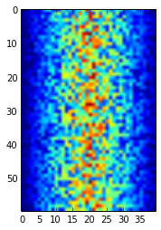

Blue regions in this heat map are low values, while red shows high values. As we can see, inflammation rises and falls over a 40-day period. Let's take a look at the average inflammation over time:

ave_inflammation = data.mean(axis=0)
pyplot.plot(ave_inflammation)
pyplot.show()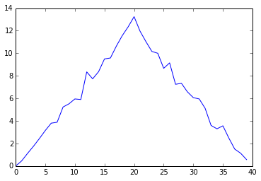

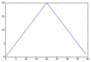
Here, we have put the average per day across all patients in the variable ave_inflammation, then asked pyplot to create and display a line graph of those values. The result is roughly a linear rise and fall, which is suspicious: based on other studies, we expect a sharper rise and slower fall. Let's have a look at two other statistics:

print 'maximum inflammation per day'
pyplot.plot(data.max(axis=0))
pyplot.show()

print 'minimum inflammation per day'
pyplot.plot(data.min(axis=0))
pyplot.show()

maximum inflammation per day

minimum inflammation per day

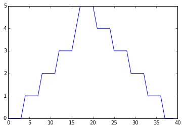
The maximum value rises and falls perfectly smoothly, while the minimum seems to be a step function. Neither result seems particularly likely, so either there's a mistake in our calculations or something is wrong with our data.

Wrapping Up

It's very common to create an alias for a library when importing it in order to reduce the amount of typing we have to do. Here are our three plots side by side using aliases for numpy and pyplot:

import numpy as np
from matplotlib import pyplot as plt

data = np.loadtxt(fname='inflammation-01.csv', delimiter=',')

plt.figure(figsize=(10.0, 3.0))

plt.subplot(1, 3, 1)
plt.ylabel('average')
plt.plot(data.mean(0))

plt.subplot(1, 3, 2)
plt.ylabel('max')
plt.plot(data.max(0))

plt.subplot(1, 3, 3)
plt.ylabel('min')
plt.plot(data.min(0))

plt.tight_layout()
plt.show()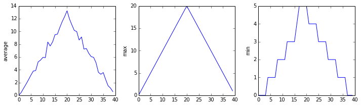

The first two lines re-load our libraries as np and plt, which are the aliases most Python programmers use. The call to loadtxt reads our data, and the rest of the program tells the plotting library how large we want the figure to be, that we're creating three sub-plots, what to draw for each one, and that we want a tight layout. (Perversely, if we leave out that call to plt.tight_layout(), the graphs will actually be squeezed together more closely.)

Next Steps

Our work so far has convinced us that something's wrong with our first data file. We would like to check the other 11 the same way, but typing in the same commands repeatedly is tedious and error-prone. Since computers don't get bored (that we know of), we should create a way to do a complete analysis with a single command, and then figure out how to repeat that step once for each file. These operations are the subjects of the next two lessons.